Visually Do Shape Analysis !
by Prof. Yukari Shirota (Gakushuin Univ., Japan),
Prof. Riri Fitri Sari (Univ. of Indonesia),
Dr.Tetri Widiyani (Sebelas Maret University, Indonesia), and
Prof. Takako Hashimoto (Chiba University of Commerce, Japan),
Abstract: Recently a new morphometric statistical analysis has been growing.
This analysis was developed by the University of Leeds in 1998 called statistical shape analysis or commonly known
as geometric statistics. Using this statistical analysis we can measure the change in the shape of an object or
so-called deformation, easily. The problem on transforming data sets in the different size, orientation and shape
of an object into a coordinate system had been very difficult, over years.
By this analysis, we can be quantified the shape of an object by eliminating information of location,
rotation, and scale. However, the mathematics is a bit difficult to understand.
To solve the problem, this teaching material web site.
Here we will explain the math process visually. Visualization has the power to make people
understand the content meaning at a glance. The visualization power is required in mathematics education.
We have developed and used many visual teaching materials for our university math lectures.
The teaching materials of the shape analysis have developed
as a joint research project result of Japan and Indonesia researchers.
They are Prof. Yukari Shirota (Gakushuin Univ., Japan), Prof. Takako Hashimoto (Chiba University of Commerce, Japan),
Prof. Riri Fitri Sari (Univ. of Indonesia), and Dr.Tetri Widiyani (Sebelas Maret University, Indonesia).
The project was supported by the Computer Centre of Gakushuin Univ. as a 2017 special rsearch project.
Using the teaching materials, we will do the tutorial lectures in
IEEE DSAA (Data Science and Advanced Analysis) 2017
to be held on 19-21, Oct. 2017 in Tokyo.
We would like to explain the mathematics visually and interactively.
We hope that the readers access the visual materials for themselves.
The graphics were written in Wolfram CDF. With the free software �$B!H�(BWolfram CDF player�$B!I�(B
everyone can operate the graphics.
In addition, we eagerly hope that more people who need mathematics enjoy the mathematics
using the visual materials.
REFERENCES
1.	Dryden, I.L. and K.V. Mardia, Statistical shape analysis with Applications in R (Second Edition). 2016: J. Wiley Chichester.
2.	Mardia, K., F. Bookstein, and J. Kent, Alcohol, babies and the death penalty: Saving lives by analysing the shape of the brain. Significance, 2013. 10(3): p. 12-16.
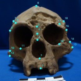
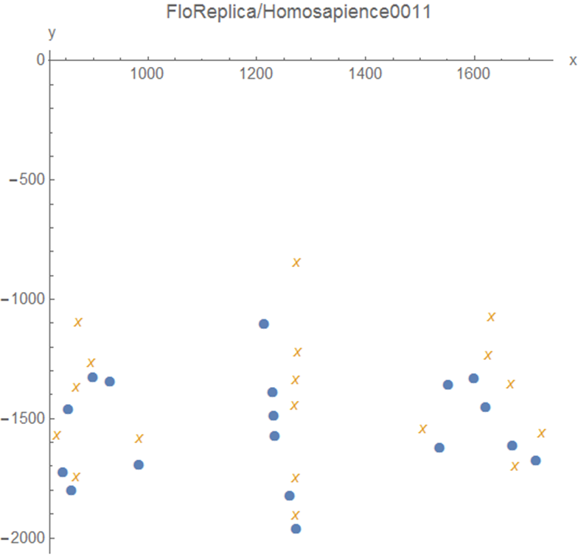
(1) Deformation between Homo floresiensis and Homo sapience
Figure 1: Homo floresiensis (left, blue) and
Homo sapiens (right, yellow)
photos with the 18 landmarks and the two configurations (centre).
First, let us show the interesting analysis results to the audience
so that the audience can understand the goal of the shape analysis.
Let's see the craniofacial differences of the two ancient humans;
they are Homo floresiensis (left) and Homo sapiens (right)
(See Figure 1).
We would like to thank the Director Sukronedi (S.Si, M.A.) and staff members of Sangiran Early Man Site Museum,
Indonesia for giving us a permission of an access to the ancient human craniofacial collections.
In Indonesia, we can discover various bone fossils of early men, including craniofacial bones,
especially in the vicinity of Solo city, Indonesia.
Concerning Homo floresiensis, controversial discussion has occurred,
when Homo floresiensis was found in an isolated island named "Flores" in Indonesia.
In the materials, let us see the local changes between the two early men's photos
using the statistical shae analysis.
We set the 18 landmarks are given on a skull photo.
The same number means that they are corresponding positions.
We would like to analyse the local movements/changes between the corresponding landmarks.
For example, the forehead became wider or the chin was getting smaller.
Using the shape analysis, we can divide the deformation to the Affine transformation and
non-Affine transformation.
The Affine transformation can express how the total plane change is such as skewing. However,
the Affine transformation cannot express the local movements.
The local movements can be expressed as a non-Affine transtformation.
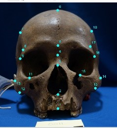
Figure 2: The deformation of the two pre-shapes.
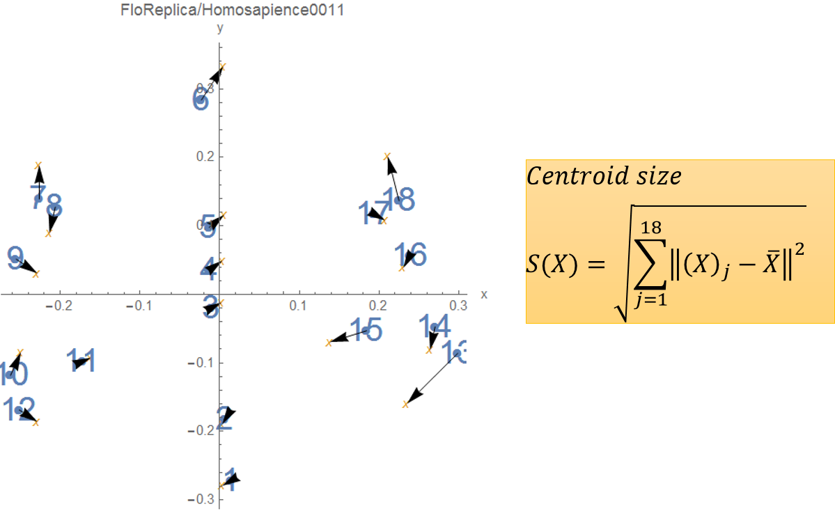
First, the given condiguration must be moved to the centre (centering) and then divided by the centroid size
(scaling). The resulting shape is called a pre-shape.
Figure 3: The deformation is divided to Affine and non-Affine transformations.
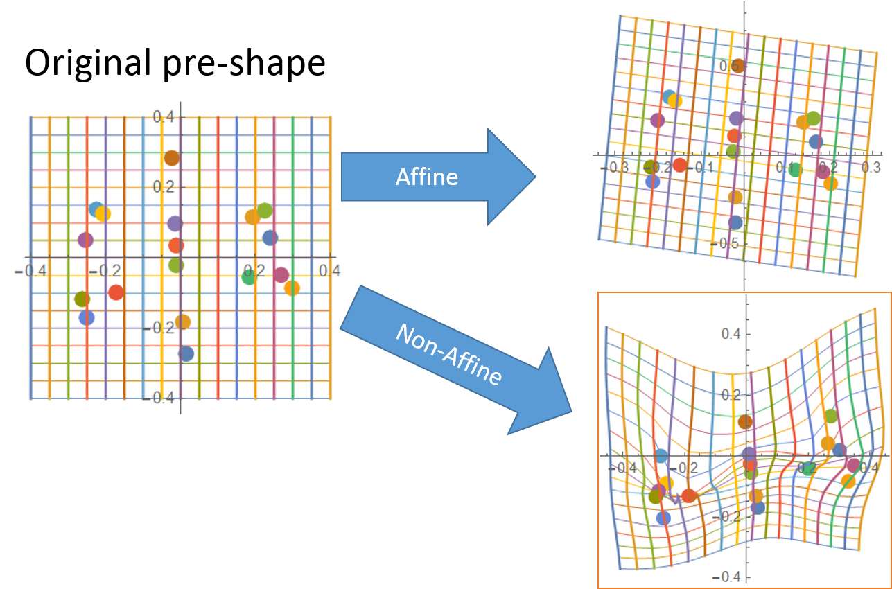
The deformation in Figure 2 is divided to the Affine and the non-Affine transformations.
Figure 4a: A pair of thin-plate splines for the deformation.
(OPEN graphics)
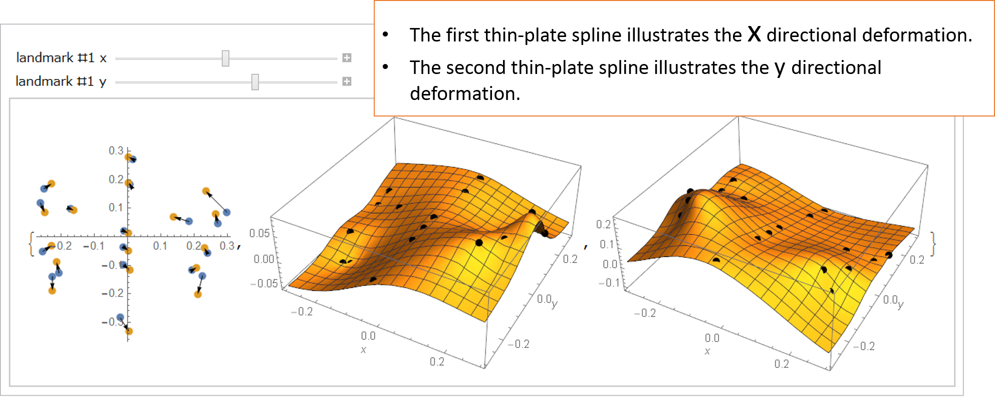
The deformation can be mathematically expressed by a pair of thin-plate splines.
The deformation include both the Affine and non-Affine transformations.
Let's open the graphics which needs in advance to install the Wolfram CDF player.
In the graphics, there are two sliders by which you can move the #1 landmark position
x and y. When you change the x value of the #1 landmark, only the first spline will be changes.
Let us change the x value to be positive and negative; then the point of the first spline surface will
go up and down. We think that this interactive operation on the graphics would make you surely understand
the math.
Figure 4b: Spline base functions make the thin-plate splines.
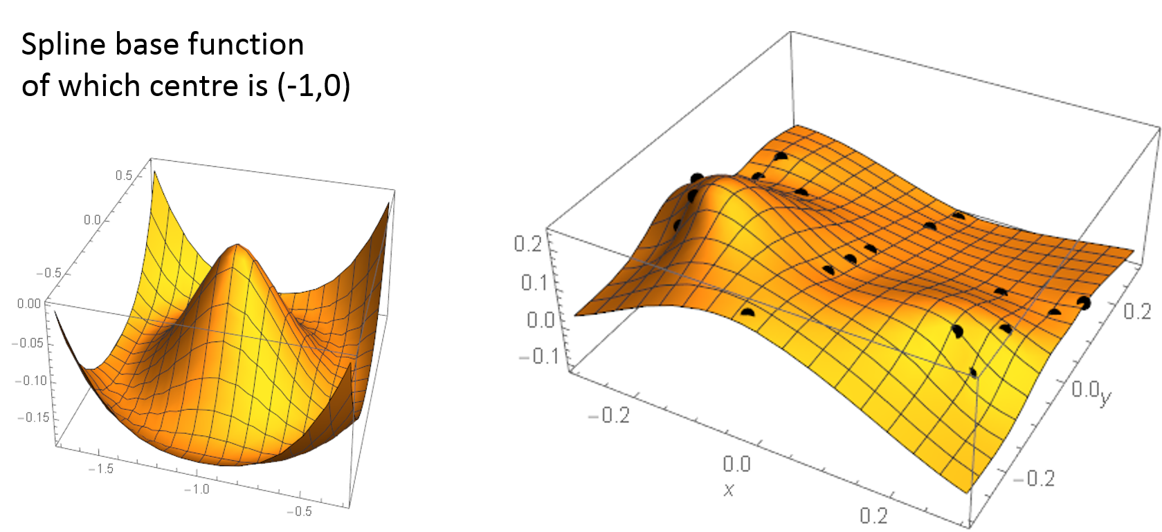
Let us explain how to make the spline surface.
The interpolation can be made by Spline base functions.
The function has the just one local maximum point. We set the point
at each landmark position. Then we find the minimum point so that
the total landmark points would be connected most smoothly.
The resultant interpolation is displayed in the graphics. At the
time, the bending energy of the pair of thin-plate Splines is minimum.
Figure 5a: The top 6 principal warps of the Homo floresiensis' (left) preshape.
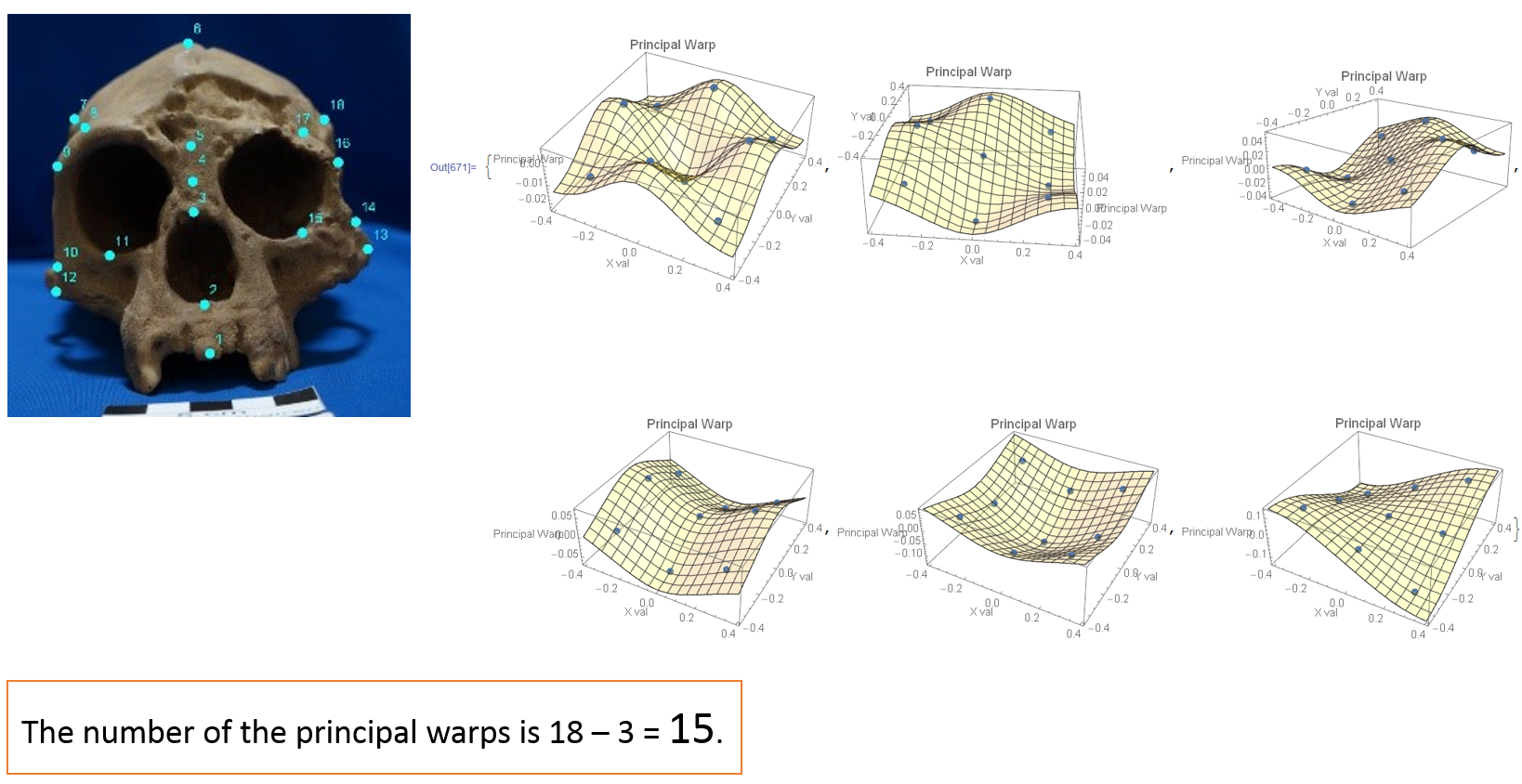
Given a photo with landmarks, we can obtain the foundamental characteristics
of the landmark layout. First we make a bending energy matrix of the given
shape and calculate the eigenvectors of the matrix.
Later, we shall explain the bending energy matirx.
The individual eigenvector times (inner product) the above-mentioned Spline base functions becomes
the surface shown in Figure 5a. The surface is called a principal warp.
The eigenvalue is called the bending energy.
In Figure 5a, the principal warps of the Homo floresiensis' (left) preshape
are illustrated. The number of principal warps is 18 -3 = 15 in this case.
Because there is not enough space on the web page, only top 6 partial warps are displyed,
although the number of principal warps is 18 -3 = 15 in this case.
If you learn PCA (Principal Component Analysis), an analogy would be helpful.
Given the configuration of the landmarks, the principal components of the configuration
are extracted like this.
Figure 5b: The top 5 principal warps of the Homo floresiensis' (left) pre-shape.
(OPEN graphics)
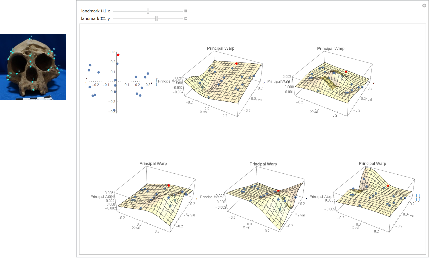
(OPEN VIDEO)
Let's move the principal warps by moving the #1 landmark which is red marked.
Please remember that the landmark movement changes the partial warps; although
you need not analyse the changing rules (The authors do not identify the changing rules, too.)
Figure 5c: The principal warp eigenvalues of the Homo floresiensis' (left) pre-shape.
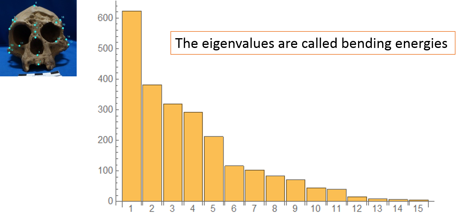
Next let's see the principal warp eigenvaues which are shown in the bar chart.
There are 15 eigenvalues. The biggest one is about 600 and the second one is about 400.
Figure 6: The top 3 partial warps of the non-Affine deformation from Homo floresiensis' to Homo sapiens.
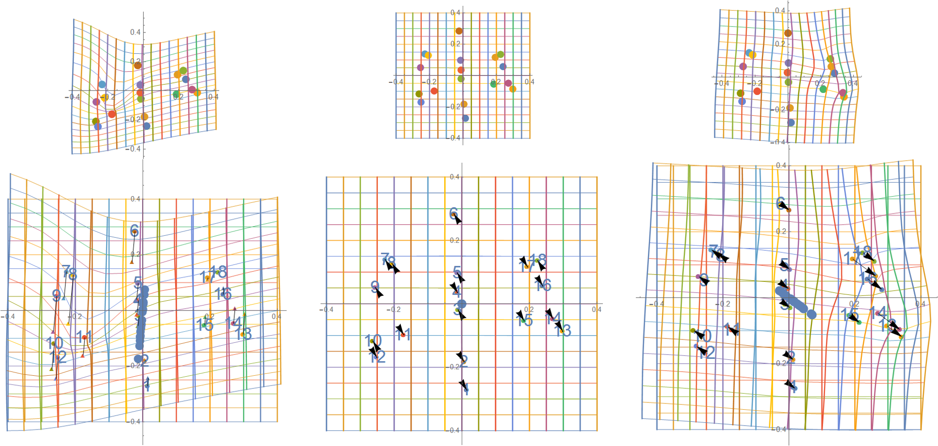
The non-Affine transforamtion of the deformation can be expressed by the
partial warps.
The partial warp is a mapping of the thin-plate spline transformations to the principal warp.
Figue 6 shows the partial warps of the non-Affine formation from Homo floresiensis' to Homo sapiens.
From left to right, the first partial warp to the third partial warp are illustrated.
In each figure, both the original shape and the partial warp are shown.
The differencial vector of each landmark lines up on a straight line (See the
centre of each figure around the origin).
In the shape analysis, the partial wapr is important. The partial warp can give us
which landmarks changes much or less and the change directions.
In figure 6, no big change can be seen in the second partial warp.
(2) Deformation between a relaxed cat and an angree cat
Figure 7: When a relaxed cat gets cross and arches its back, the 9 landmarks get nearer to the centre.
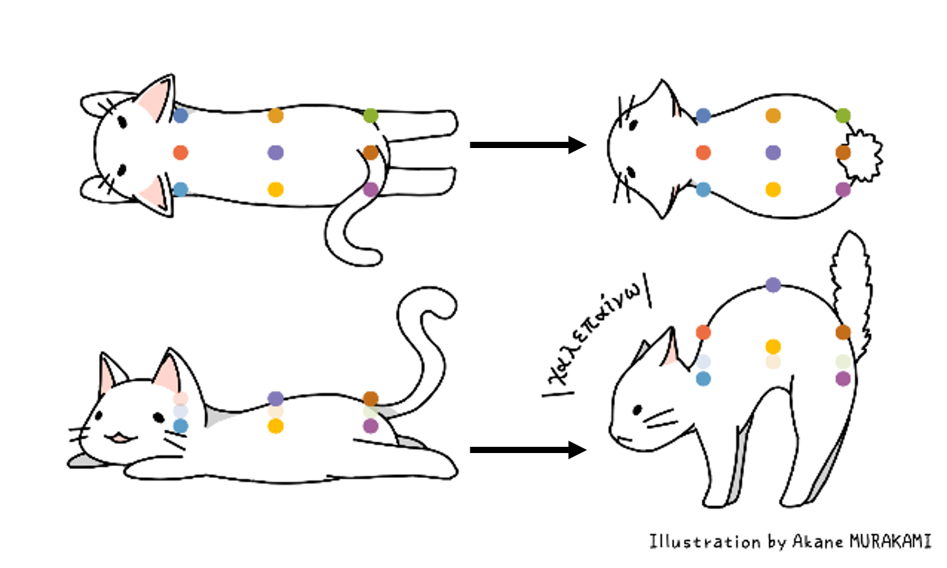
In the section, using a simple deformation, the math process will
be explained visually. In the section, a shape, not a pre-shape, is
used.
Figure 8: The deformation of the flatten can got cross. (non pre-shapes)
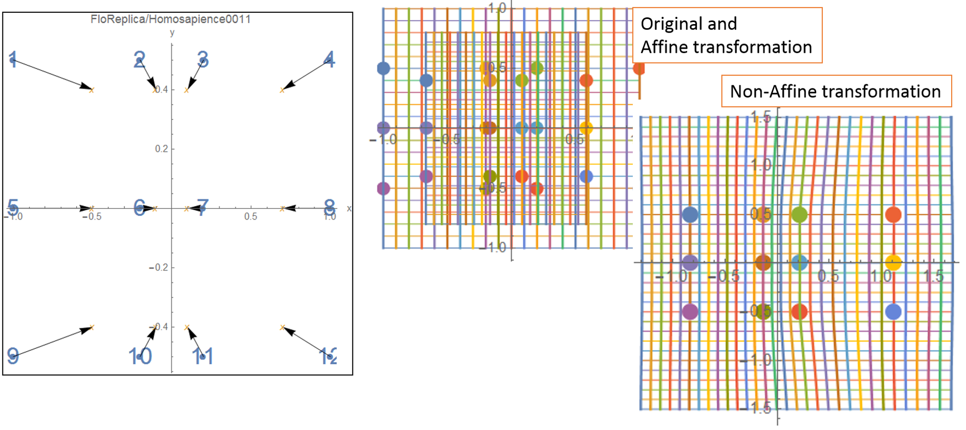
As shown in Figure 8, we plot the 12 landmarks on the cat back.
In Figure 6, the deformation, its Affine transformation and its
non-Affine transformation are shown.
In the Affine transformation, we can see the shrink of the
transformation grids.
In the non-Affine tansformation, we cann see the local movement
of the 6 landmarks at the centre.
Figure 9: Thin-plate spline interpolation of the cat deformation.
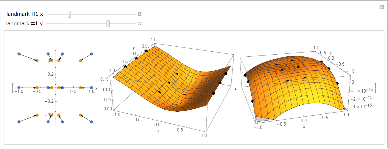
The deformation can be expressed by a pair of thin-plate splines.
Figure 10: Bending energy matrix of the relaxed cat.
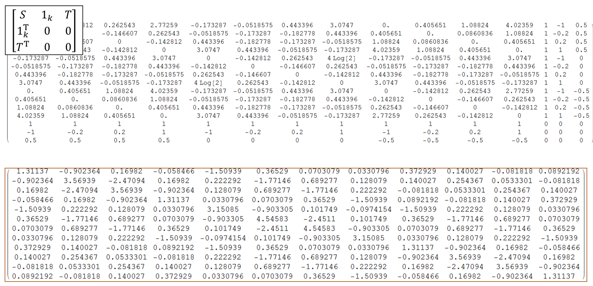
Let's calculate the bending energy matrix of the relaxed cat.
Figure 10 shows two matrices. First, we make the first matrix.
The matrix S of which size is 12 times 12 is calculated by the spline base function.
The matrix T is the given shape T; in the case, the shape of the relaxed cat.
Then we calcurate the inverse matrix of this matrix.
Next, take the right-upper part of which size is 9 times 9. This is the bending
energy matrix (See the matrix at the bottom).
Figure 11: The relaxed cat�$B!G�(Bs 9 principal warp eigenvalues and 2 eigenvectors.
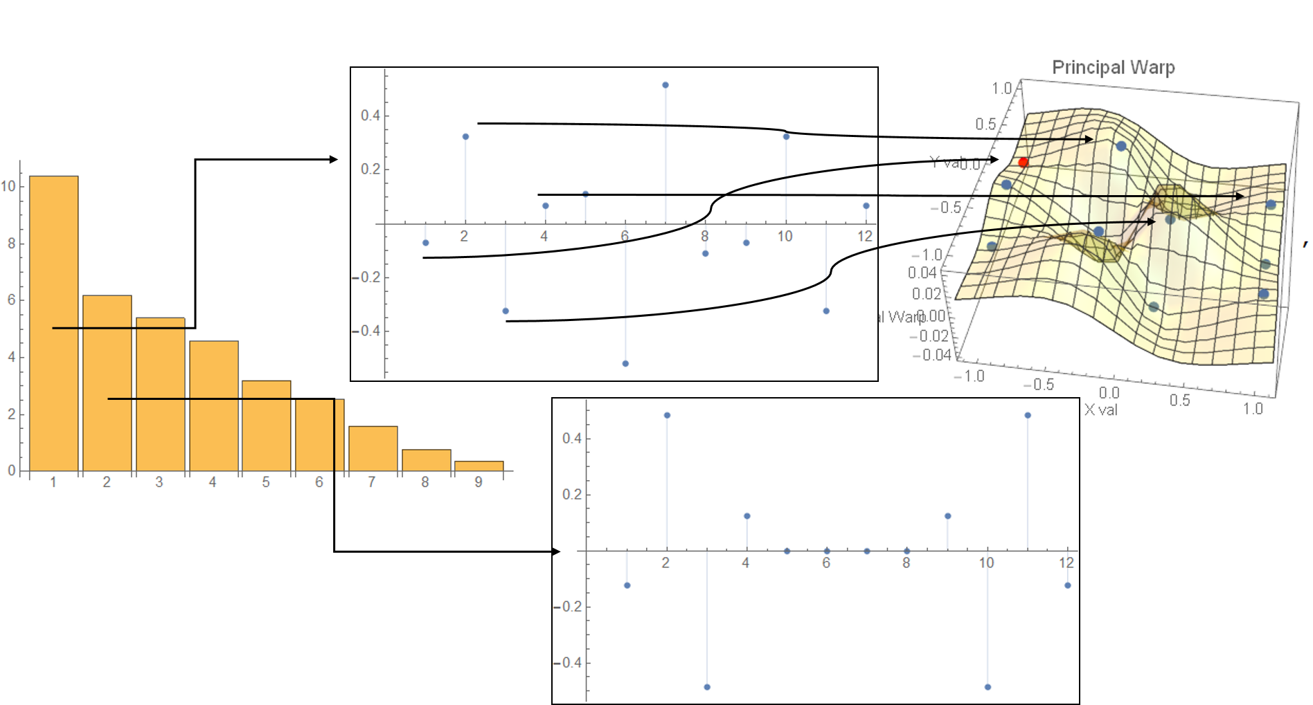
Next let us calculate the eigenvalues and eigenvectors of the bending energy matrix.
In the left figure, the bar char of the eigenvalues are shown. There we can see
the biggest eigenvalue is about 10 and the second one is nearly 6.
In the center of the figure, two eigenvectors are shown. The upper one
shows the first eigenvector which consists of 12 factors.
Each factor shows each landmark's contribution to the first partial warp;
the red marked landmark's factor value is negative about -0.06 so the point
becomes a valley in the spline surface. Concerning the second landmark,
the factor value is about 0.3 so the point becomes a mountain.
Figure 12: The relaxed cat's first principal warp.
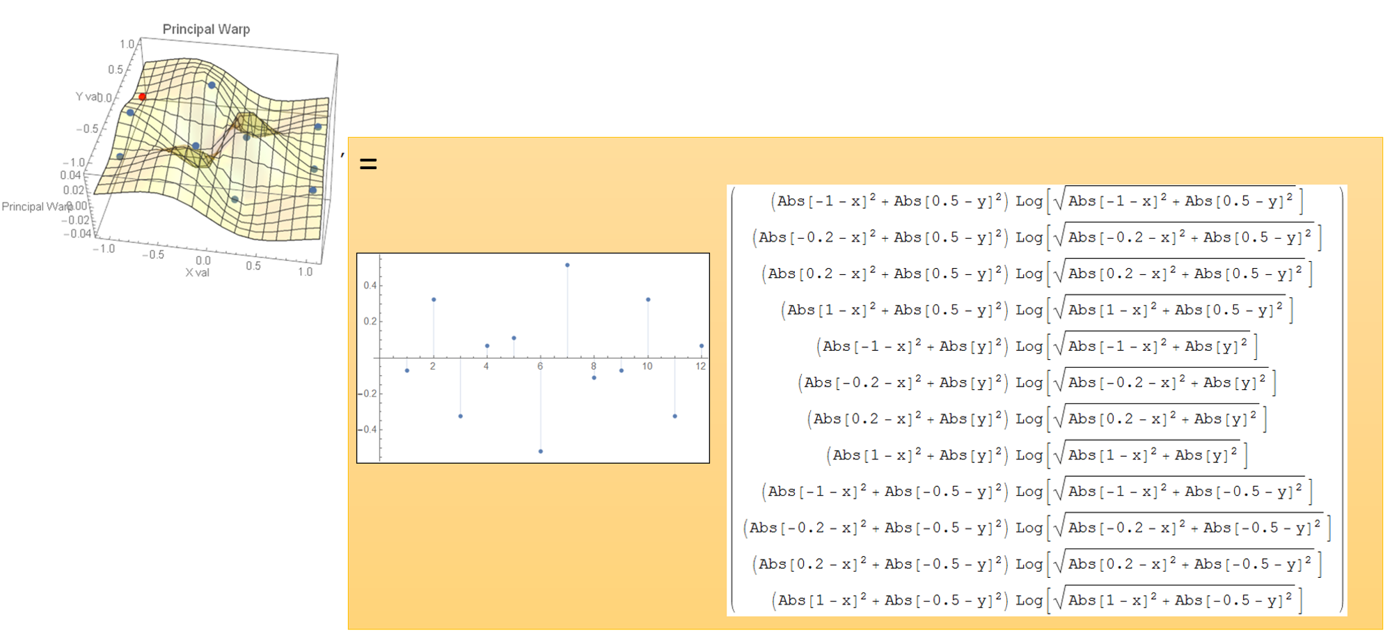
Let's see the function of the first principal warp (See Figure 12).
That is a inner product of the eigenvector and the spline base functions
at each landmark positions.
Figure 13: The 6th partial warps of the deformation
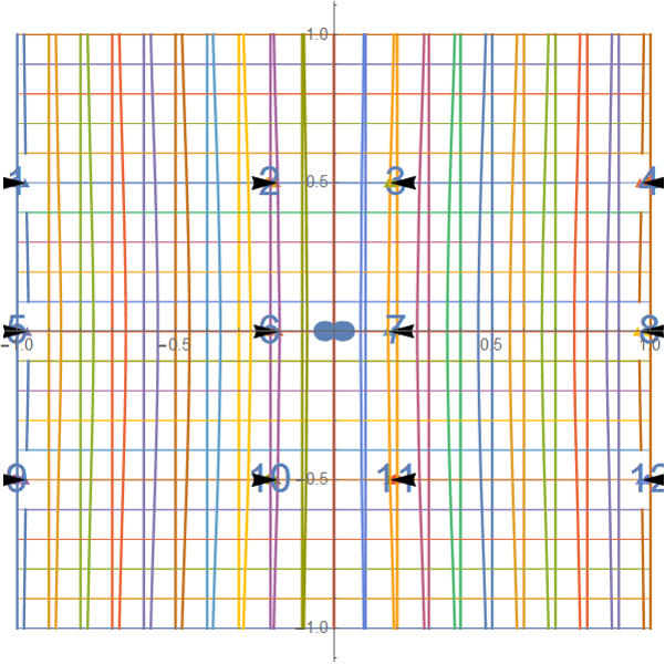
Finally, the partial warps of the deformation are shown.
Although we can obtained the 9 partial warps, the first to the
fifth partial warps did not show a large local movements, just a
subtle change. In the sisth partial warp, we fist identified the
local movement as shown in Figure 13. They are horizontal directional
movements. As shown in the above, the scaling changes
are involved in the Affine transformation.
We shall conclude the materials here. We explained the parial warps of
the shape analysis. In addition, explanations of the analysis of variance (ANOVA) would be needed.
However, the ANOVA is lectured in statistics lectures. So we skip the ANOVA.
The most surprising point of the shape analysis is discovery of the
principal warps from the bending energy matrix, the authors think.
Every time we use the shape analysis method, we wonder how was it inspired
so that they would have the idea of the bending energy matrix.
We are interested in an economics data analysis, too. So we are conducting
some researches on the economics data such as stock prices.
We hope that much more researchers in various fields leverage the new analyis
method.
Authors:
(1) Yukari Shirota, DSc.
Prof. of Faculty of Economics, Gakushuin University, 1-7-1 Mejiro, Toshima-ku, Tokyo, Japan
yukari.shirota@gakushuin.ac.jp
Research fields are visualization of data on the web, social media analysis, and visual education methods for business mathematics.
1. Yukari Shirota: "Selected graphics and papers",
http://www-cc.gakushuin.ac.jp/~20010570/mathABC/SELECTED/
2. Yukari Shirota: "Mathematics Graphics Materials",
http://www-cc.gakushuin.ac.jp/~20010570/mathABC/ABC/
Others are:
http://www.gakushuin.ac.jp/univ/eco/english/teacher/sirota.html
http://www-cc.gakushuin.ac.jp/~20010570/VDStat/
(2) Dr. Ir. Riri Fitri Sari MM MSc
Prof. of Department of Electrical Engineering, Faculty of Engineering, University of Indonesia, Kampus Baru UI, Depok 16424, Indonesia, riri@ui.ac.id.
Her current main teaching and research area includes Computer Network, Protocol Engineering, Network Computing, Sustainability in Higher Education, Applications of ICT for Humanities.
(3) Dr. Tetri Widiyani
Tetri Widiyani is a Senior Lecturer at the Department of Biology of the Sebelas Maret University (UNS), Solo, Indonesia. She was awarded with a PhD from Biology from Bogor Agricultural University, IPB, Bogor, Indonesia. She is an editor of some Journals in Biology in Indonesia.
(4) Takako Hashimoto, Ph. D.
Prof. of Faculty of Commerce and Economics, Chiba University of Commerce 1-3-1, Konodai Ichikawa City, Chiba, Japan
takako@cuc.ac.jp
Chair, IEEE Women In Engineering (2015)
Coordinator, IEEE R10 Women In Engineering (2011-2014)
Past Chair, IEEE Japan Council Women In Engineering (2012-2013)
Visiting Researcher, UCLA (2015)